Read processing algorithms

*The interpretation of the Algorithm part is only available in EN.

Gene Expression Count during SAW count, for the FASTQ data from the Stereo-seq sequencing platform, includes the following analysis stages:

Regarding the key steps of read alignment and annotation, a flowchart is used to illustrate.

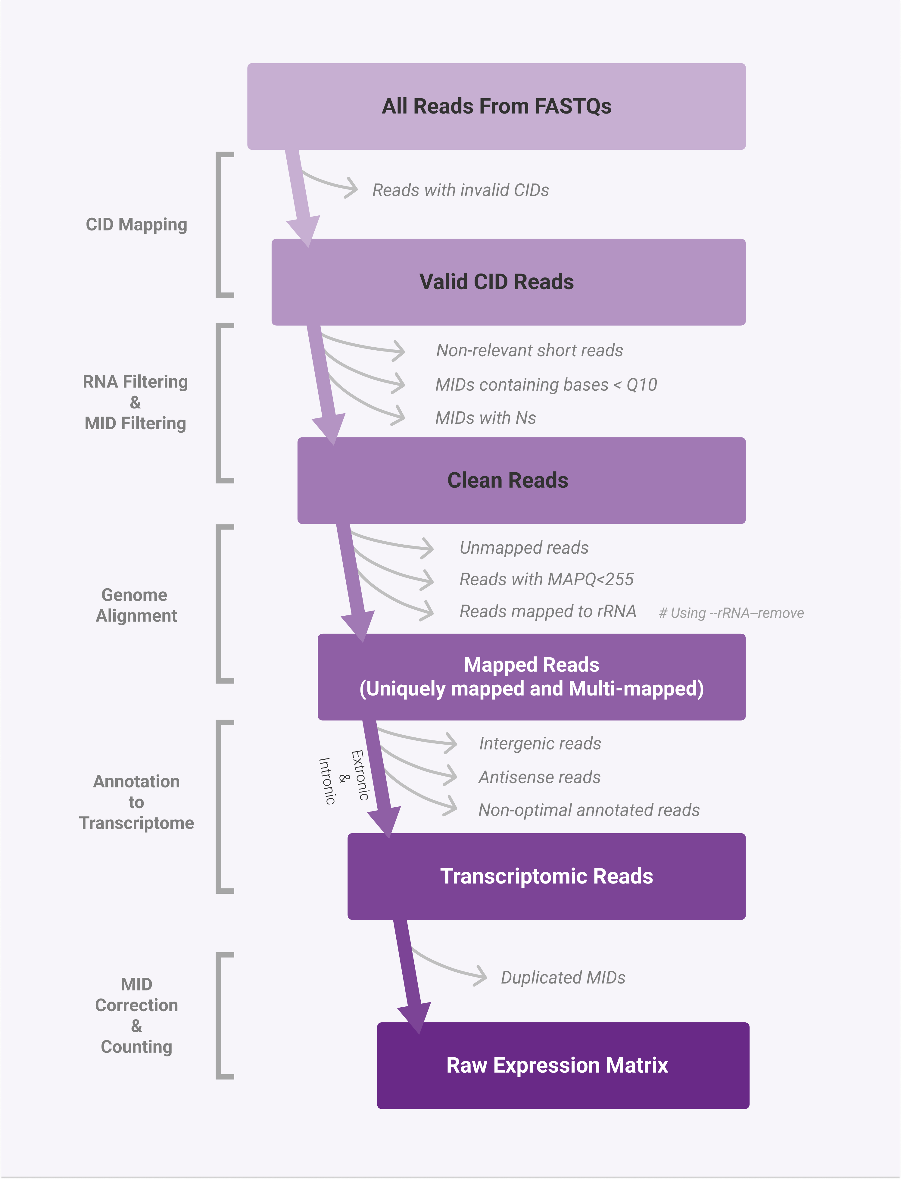
Alignment & Annotation

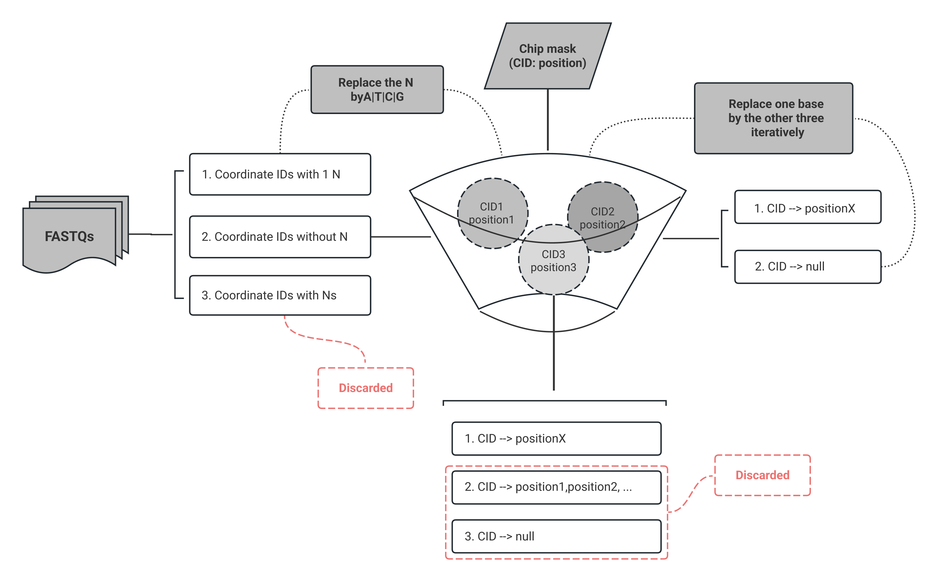
CID mapping

CID mapping requires FASTQs and a chip mask file, recording position information for sequencing reads.

Check the amount of Ns in Coordinate IDs:

• If there is 1 N base in CID, the N base will be replaced by A/T/C/G.
• CIDs without N bases will be directly poured into the match pool.
• CIDs with more than one N base will be discarded.

In the absense of an N base, if a CID does not match to any positions, each base of the CID will replaced by the other three types iterately until a successful match. After the mapping, only the unique CID match will be retained for subsequent steps.

RNA filtering

Before genome alignment, it is necessary to confirm that the reads entering the next step are cDNA sequences. Ideally, this part of the data only contains cDNA fragments, but there may be cases where the fragmented cDNA is too short or some non-cDNA fragments are detected.

Reads will be discarded if any of the following conditions are triggered:

• with a length of less than 30 after cutting out adapter sequences,
• mapped to DNB sequences,
• with a length of less than 30 after cutting out the poly-A sequence.

The above three are collectively known as "non-relevant short reads".

MID filtering

MID sequences will be filtered out if they match any of the following:

• having more than one base with quality <= Q10,
• having N bases >= 1.

Genome Alignment

To align reads to the genome with splicing awareness, SAW utilizes the STAR aligner. Using a transcript annotation GTF/GFF file, the system classifies reads as exonic, intronic, or intergenic ones based on their alignment. If a read shares at least 50% of its overlap with an exon, it is considered exonic XF:i:0. If a sequence does not meet the criteria for exon but crosses an intron, it is called intronic XF:i:1.

The exonic locus is given priority, and the read is deemed to be reliably mapped to the exonic locus with a MAPQ of 255 for reads that align to one exonic locus but also to one or more non-exonic loci.

Annotation to transcriptome

In SAW, reads mapped to exonic and intronic regions are to be annotated, using the transcriptomic annotation file.

Remove rRNA

The preconditions for rRNA filtration are:

• switching --rRNA-remove on when runningSAW count,
• addition of rRNA information to the index files using SAW makeRef.

Reads mapped to rRNA regions will have a tag of XF:i:3, and they will not move on to the next step.

Transcriptome

SAW estimates whether there is a successful annotating record based on the position of each read mapped to the genome and whether the alignment is located in a gene region.

• When the alignment direction of the read on the genome is consistent with that of a gene and overlaps with the gene >= 50% of the mapped length, the read will be considered to be annotated with the gene.
• If a read is annotated to multiple genes, the one with the longest overlap length with the gene is selected as the final result of the read. When the overlap lengths are the same, the read is considered to be annotated unsuccessfully.

Annotating types are classified according to the following rules:

• If the overlap between read and exon is >=50%, the read is considered to originate from the exonic region of the gene, otherwise, it originates from the intron region.
• Reads overlapped with genes but have inconsistent directions are classified as antisense XF:i:4.
• Reads that can be aligned to the genome but cannot be classified as gene or antisense are considered to be intergenic XF:i:2.

MID correction & counting

At a position, if the MID counts of a certain gene >= 5, they will be corrected. After sorting the MID counts of a specific gene in descending order, the numerical values are corrected following the fundamental principle that allows a Hamming distance of 1. After correction, a tag of UB:Z:XXXXX will be added to the record.

PID mapping

Check the number of N in 15bp ADT reads.

1. If the number N is greater than 1, discard the read;
2. If the number N is 1 and pidMismatch > 0, replace N with A/T/C/G, and then compare with the protein panel respectively. If the query is successful, note CNT = 1. After the iterative query is completed, if CNT = 1, perform pid_mapped_mismatch_reads++. If CNT != 1, discard the read directly.
3. If the number N is 0 and pidMismatch = 1, replace any one position of PID with the other three bases for the query. If the number of successful queries is 1, note CNT=1 and perform pid_mapped_mismatch_reads++. If the number of successful queries exceeds 1, note CNT != 1, and discard the read.

Secondary analysis

The secondary analysis, in SAW count and SAW realign, are performed using Stereopy. The procedure includes 6 main parts:

• Preprocess gene expression data from the tissue coverage region (normalize, logarithmize, identify highly variable genes, and scale each gene).
• Reduce the dimensionality of the data by running PCA.
• Compute the neighborhood graph and embed the neighborhood graph using UMAP.
• Clustering by Leiden algorithm.
• Perform differential expression analysis, using the t-test to find marker features.
• Output analysis result file in AnnData H5AD and marker feature CSV.

Dimensionality reduction

PCA: Spatiotemporal transcriptome data often contain thousands of genes, making the data high-dimensional and challenging to analyze. Principal Components Analysis (PCA) reduces dimensionality by transforming the data into a set of principal components (PCs) that capture the most significant variance.

UMAP: SAW supports Uniform Manifold Approximation and Projection (UMAP), which is a popular non-linear dimensionality reduction technique that is particularly useful for visualizing high-dimensional data in a low-dimensional space. In the context of spatiotemporal transcriptome data analysis, it is beneficial to capture both local and global structures as it facilitates the interpretation of complex datasets. UMAP coordinates are available in the pipeline output H5AD, as well as being displayed in the HTML report and StereoMap.

Clustering

SAW uses Leiden algorithm for clustering spots by expression similarity, operating in the PCA representation.

Leiden: an algorithm for network community detection, which is particularly important in bioinformatics analysis, especially in the analysis of spatial transcriptomic datasets. It is an enhanced version of Louvain's method, developed to address its potential instability and provide higher resolution and a more robust community structure. In bioinformatics, the primary roles and benefits of Leiden algorithm can be summarized as follows:

• Improved resolution and stability: the algorithm can effectively identify smaller community structures, which is crucial for understanding cellular heterogeneity and subtle changes in complex biological processes. Compared with Louvain's method, Leiden can offer more consistent and stable results across multiple runs.
• Efficient cell type identification: in the analysis of spatial transcriptomic sequencing data, Leiden clustering can assist researchers in identifying various cell types or states from thousands of cells. By constructing a network of cell similarities, Leiden algorithm can cluster similar cells together to form distinct groups, which typically correspond to various biological functions or cell types.
• Powerful community structure detection: Leiden algorithm ensures the quality of clustering by optimizing a modularity function, which helps reveal complex biological patterns and potential regulatory networks in samples. It is particularly important for understanding the interactions and signal transduction pathways between cells.
• Applicable to large-scale datasets: with the advancement of single-cell sequencing technology, the size of datasets is increasing. The Leiden algorithm's computational efficiency allows it to handle large-scale datasets while keeping computational costs low.
• Flexibility and scalability: it is not only applicable to spatial transcriptomic data but can also be extended to other types of bioinformatic data, such as protein interaction networks, metabolic networks, etc.

Differential expression

To identify genes whose expression is specific to each cluster for each gene and each cluster, whether the in-cluster mean differs from the out-of-cluster mean.

t-test: the method used in the find_marker_genes of Stereopy package is based on classical statistical principles to identify differentially expressed genes between groups of cells.

• Grouping cells: cells are grouped based on a categorical variable, such as cluster labels obtained from the Leiden clustering algorithm. For example, cells in cluster A are compared to cells in cluster B.
• Expression levels: for each gene, the expression levels are compared between the two groups of cells.
• Calculating the t-statistic: the t-statistic is calculated using the formula:

• Degrees of freedom: the degrees of freedom (df) for the test are calculated, often using a formula that takes into account the sample sizes and variances of both groups.
• P-value calculation: the t-statistic is then compared to the t-distribution with the calculated degrees of freedom to obtain a p-value. This p-value indicates the probability that the observed difference in means could have occurred by chance.
• Multiple testing correction: given that thousands of genes are tested simultaneously, multiple testing correction methods (such as Benjamini-Hochberg) are applied to control the false discovery rate (FDR).

The t-test method in find_marker_genes leverages the principles of hypothesis testing to identify genes that are significantly differentially expressed between predefined groups of cells. This method provides a straightforward and statistically sound approach to uncovering key marker genes that distinguish between cell types or conditions, facilitating deeper insights into the underlying biology of the dataset.

Proteome & Transcriptome joint analysis

Combining gene and protein data allows us to gain a more comprehensive understanding of cellular identity, as these two perspectives offer different insights into the molecular state. However, it is important to consider the unique sources of technical bias and noise associated with each data type. Specifically, protein data is prone to inherent technical background noise caused by non-specifically bound antibodies. To address these challenges, we utilize Total Variational Inference (totalVI)[1], which employs a deep generative model to learn a joint probabilistic representation of paired gene and protein measurements. This approach effectively accounts for the distinct noise and technical biases of each modality. Within this framework, our tool, SAW, leverages totalVI to generate a joint latent representation of spots (or cells), produce denoised gene and protein data, and compute differential expression of gene and protein.

To initiate the totalVI model, SAW inputs matrices of gene and protein unique molecular identifier counts (GEF file) for spots or cells. The model then generates a joint low-dimensional latent space. For cluster identification, SAW employs the Leiden algorithm and visualizes the clusters using UMAP. Differential expression testing (DE test) is conducted using totalVI, which estimates a distribution over the log fold change (LFC) of expression between two sets of spots (or cells). This distribution is utilized to quantify the strength of evidence supporting a hypothesis of differential expression, employing Bayes factors. SAW performs a one-vs-all DE test to determine gene and protein markers for each cluster, respectively, and stores the results in a single dataframe in CSV format. To filter the results, we retain features with a Bayes factor on the natural log scale above a specified threshold (>1 for gene markers, >0.7 for protein markers), as well as genes with an expression proportion greater than 10% in the cluster of interest. The denoised gene and protein data are produced in the H5MU format, allowing for visualization of gene and protein markers within each cluster using a heatmap.

Proteome background removal

There is non-specificity in protein antibody binding to cell surface antigens in tissues. Therefore, the antibody protein signal intensity detected in the tissue includes two situations:

• Protein positive signal is specific binding;
• Protein negative signal is non-specific binding.

Therefore, it is necessary to dynamically determine a reasonable threshold to distinguish protein positive signals from negative signals. Different antibody protein thresholds are independent of each other and do not affect each other, and the threshold must meet the following conditions:

• The intra-class variance of the protein positive signal set and the negative signal set is the smallest
• The inter-class variance of the protein positive signal set and the negative signal set is the largest

In order to complete the above conditions, it is necessary to perform：

1. Remove the duplicates of the protein signal intensity and sort it from small to large, noted as (m1, m2, m3, m4, ..., mn), and then count the frequency of occurrence of each signal intensity m, noted as (f1, f2, f3, f4, ..., fn).
2. Set the initial threshold t, and t satisfies m1 < t < mn. Then take t as the threshold, classify those greater than t into one category, note them asC1. Those less than or equal to t are classified into one category, noted as C2. Then calculate the inter-class and intra-class variances of C1 and C2. Since the sum of the intra-class and inter-class variances is a constant when the inter-class variance is the largest, the intra-class variance is the smallest, so only record the inter-class variance corresponding to the t value.
3. Iterate the t value and record the inter-class variance corresponding to each t. After the iteration is completed, take the t value corresponding to the maximum inter-class variance as the reasonable threshold to distinguish the positive signal from the negative signal of the protein.
4. According to the determined threshold, perform the following operations: A value greater than the threshold is considered a specific binding signal. A value less than or equal to the threshold is considered a non-specific binding signal. Then filter out the bin or cell of the non-specific binding signal to achieve background removal.

References

1. Gayoso, A., Steier, Z., Lopez, R., Regier, J., Nazor, K. L., Streets, A., & Yosef, N. (2021). Joint probabilistic modeling of single-cell multi-omic data with totalVI. Nature Methods, 18(3), 272-282.