
HTML report
*The interpretation of the HTML report is only available in EN.
SAW count and SAW realign pipelines will output an interactive report <SN>.report.html. The contents of the HTML report file will vary depending on the pipeline and parameters used but generally follow a similar format across runs.
On this page, we demonstrate the report of
- a mouse brain sample from Stereo-seq T FF V1.3,
- a mouse lung tissue sample from Stereo-seq N FFPE V1.0,
- and a mouse thymus tissue sample from Stereo-CITE T V1.0.
Run with SAW v8.1.
Summary
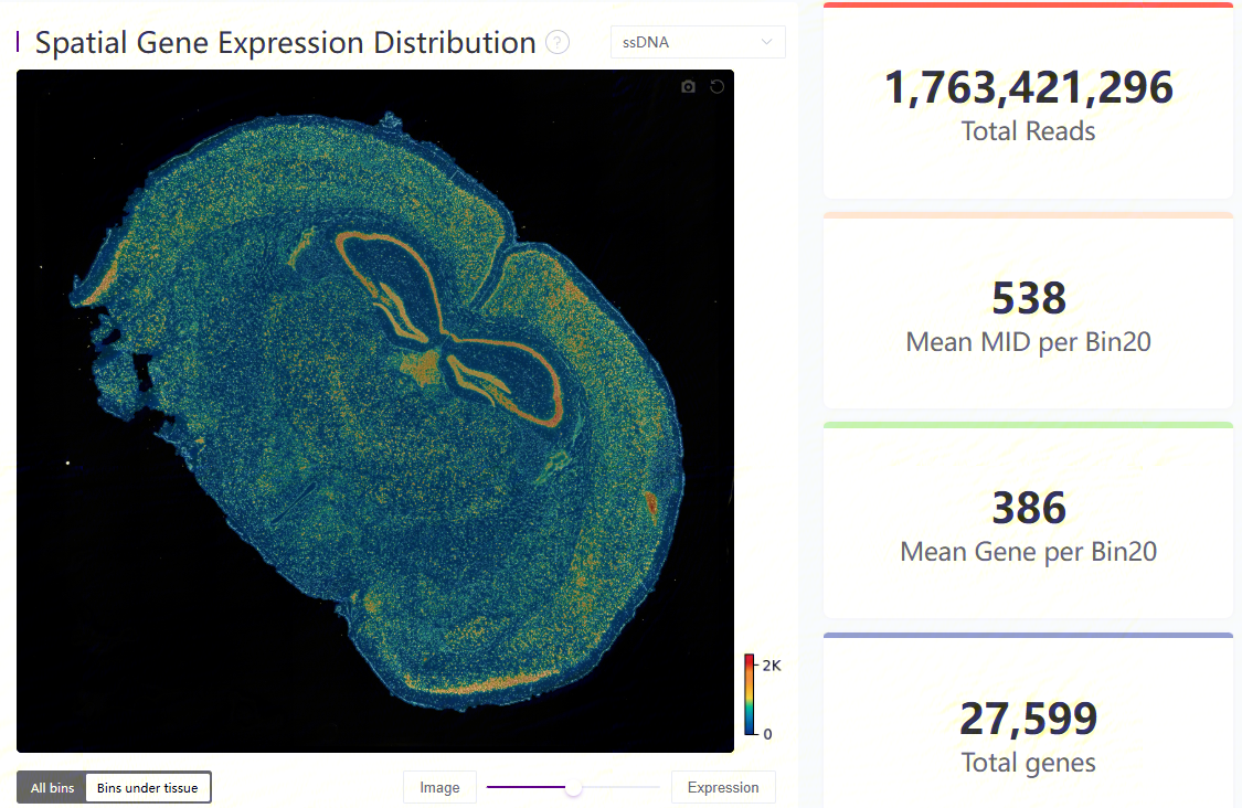
Expression heatmap and four key metrics
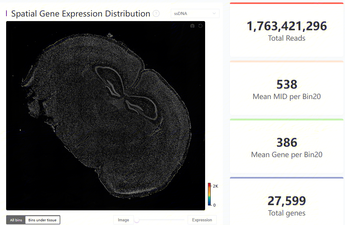
Display of microscope image
The spatial gene expression distribution plot, containing all bins and bins under tissue, on the left, shows MID count at each bin20.
Total Reads is the amount of total sequencing reads of input FASTQs. Mean MID per Bin20/Mean MID per Bin50 and Mean Gene per Bin20/Mean Gene per Bin50 represent the mean MID and gene type counts at each bin20 or bin50. Total Genes is the number of gene types from all bins.
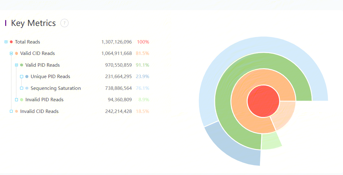
Key metrics
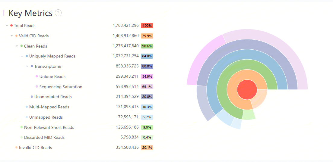
Details and sunburst plot of key metrics
Key metrics of the data are listed:
| Metric | Description |
|---|---|
| Total Reads | Total number of sequenced reads. |
| Valid CID Reads | Number of reads with CIDs that can be matched with the mask file |
| Invalid CID Reads | Number of reads with CIDs that cannot be matched with the mask file. |
| Clean Reads | Number of Valid CID Reads that have passed QC. |
| Non-Relevant Short Reads | Number of non-relevant short reads |
| Discarded MID Reads | Number of reads with MID that have been discarded since MID sequence quality does not satisfy with further analysis. |
| Uniquely Mapped Reads | Number of reads that mapped uniquely to the reference genome. If the pipeline uses uniquely mapped reads and the best match from multi-mapped reads for subsequent annotation, this item will include them both |
| Transcriptome | Number of reads that are aligned to transcripts of at least one gene |
| Unique Reads | Number of reads in Transcriptome that have been corrected by MAPQ and deduplicated |
| Sequencing Saturation | Number of reads in Transcriptome that have been corrected by MAPQ with duplicated MID |
| Unannotated Reads | Number of reads that cannot be aligned to the transcript of one gene |
| Multi-Mapped Reads | Number of reads that mapped more than one time on the genome. If the pipeline uses uniquely mapped reads and the best match from multi-mapped reads for subsequent annotation, this item will exclude multi-mapped ones to be annotated |
| Unmapped Reads | Number of reads that cannot be mapped to the reference genome. |
| rRNA Reads | Number of reads that mapped to the rRNA regions. |
Annotation
Metrics of reads to be annotated by GTF/GFF files.
| Metric | Description |
|---|---|
| Exonic | Number of reads that mapped uniquely to an exonic region and on the same strand of the genome. |
| Intronic | Number of reads that mapped uniquely to an intronic region and on the same strand of the genome. |
| Intergenic | Number of reads that mapped uniquely to an intergenic region and on the same strand of the genome. |
| Antisense | Number of reads mapped to the transcriptome but on the opposite strand of their annotated gene. |
Tissue related
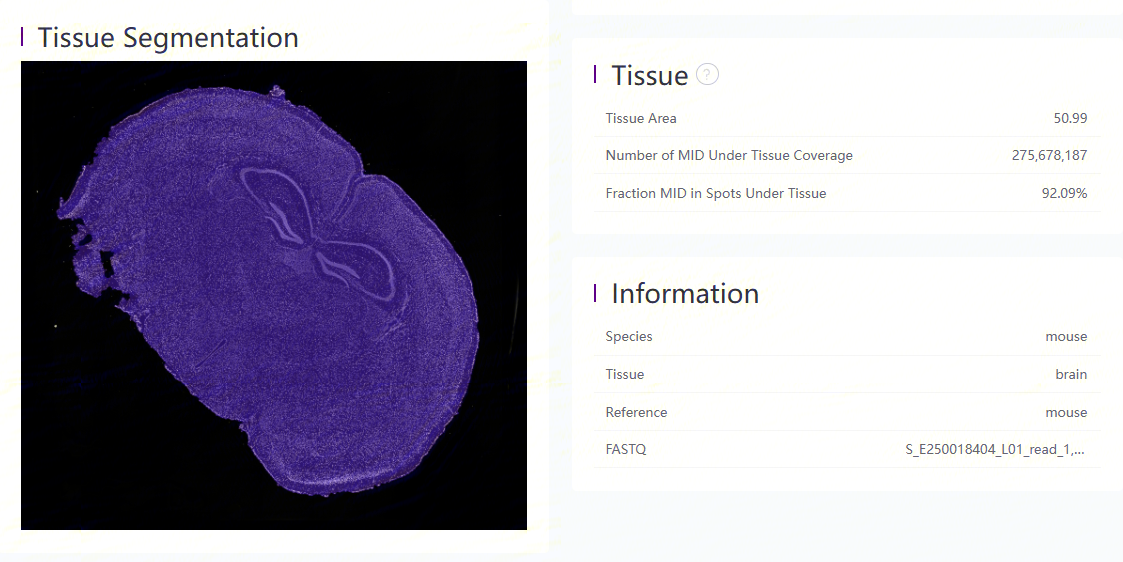
Display and metrics related to tissue-coverage region
The tissue segmentation result based on a microscope image is shown on the left, of which the tissue region is covered in purple.
Metrics related to tissue coverage are listed:
| Metric | Description |
|---|---|
| Tissue Area | Tissue area in mm². |
| Number of MID Under Tissue Coverage | Number of MID under tissue coverage. |
| Fraction MID in Spots Under Tissue | Fraction of MID under tissue over total unique reads. (MID Under Tissue / Unique Reads) |
Sequencing saturation
.PNG)
Sequencing saturation curves
The saturation analysis in the HTML report can assess the overall quality of the sequencing data. In order to improve calculation efficiency, small samples are randomly selected from successfully annotated reads in the bin20 or bin50 dimension. Therefore, the results of multiple runs of the same data may vary slightly. The formulas may not be identical, but the general shape of the curve is consistent.
- Figure 1: As the number of random samples increases, the gene median in the bin20 dimension gradually increases.
- Figure 2: Curves fitted based on Unique Reads data from randomly sampled samples.
- Figure 3: Statistics of Unique Reads (reads with unique CID, geneName and MID) in the sampled samples, saturation value = 1-(Unique Reads)/(Total Annotated Reads), as the sampling volume increases, the fitting curve becomes near-flat, indicating that the data tends to be saturated. Whether to add additional tests depends on the overall project design and sample conditions. For example, it is recommended that additional tests be performed on precious samples. The threshold value of 0.8 in the report serves as a reminder for recommended guidance.
The x-axis of the three graphs is the same, and the y-axis is divided into saturation value, gene median, and number of Unique Reads.
Information
This item displays the basic information of the input FASTQs,
Species is from the --organism parameter used in SAW count, usually referring to the species.
Tissue is from the --tissue parameter used in SAW count.
Reference means the reference genome used in SAW count, as the same as Organism.
FASTQ records FASTQ files in SAW count, including file prefixes of all input sequencing FASTQs.
Square Bin
This page contains results of statistics, plots, clustering, UMAP, and differential expression analysis, at bin dimension. Results come from the analysis based on <SN>.tissue.gef file.
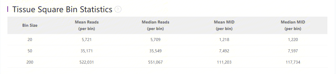
Statistics
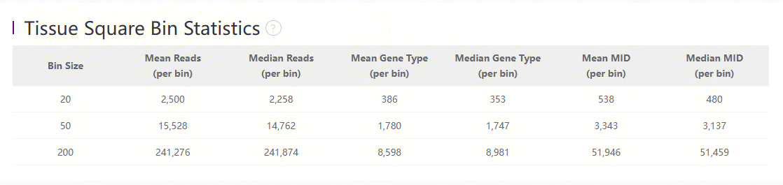
Statistics of bins under tissue-coverage region
The above table records the statistics is bin20, bin50 and bin200:
| Item | Description |
|---|---|
| Bin Size | The size of Bin which is the unit of aggregated DNBs in a squared region. i.e. Bin 50 = 50 * 50 DNBs |
| Mean Reads (per bin) | Mean number of sequenced reads divided by the number of bins under tissue coverage. |
| Median Reads (per bin) | Median number of sequenced reads divided by the number of bins under tissue coverage (pick the middle value after sorting). |
| Mean Gene Type (per bin) | Mean number of unique gene types divided by the number of bins under tissue coverage. |
| Median Gene Type (per bin) | Median number of unique gene types divided by the number of bins under tissue coverage. |
| Mean MID (per bin) | Mean number of MIDs divided by the number of bins under tissue coverage. |
| Median MID (per bin) | Median number of MIDs divided by the number of bins under tissue coverage |
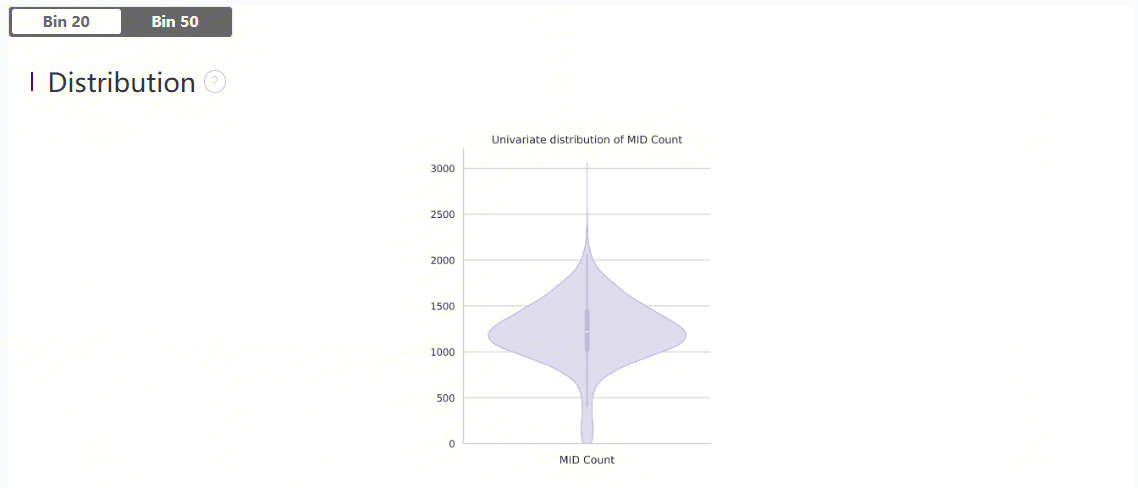
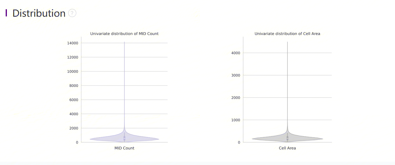
Plots
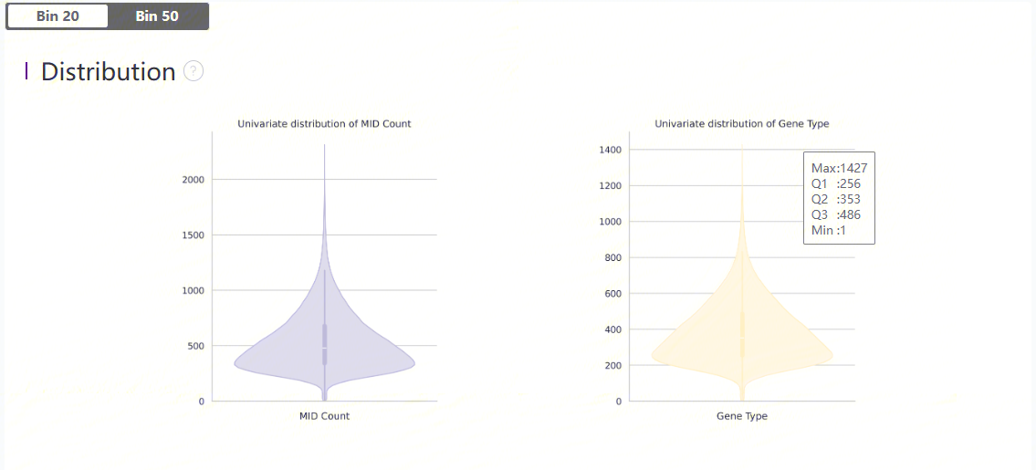
Distribution plots of MID and gene type
Violin plots show the distribution of deduplicated MID count and gene types in each bin.
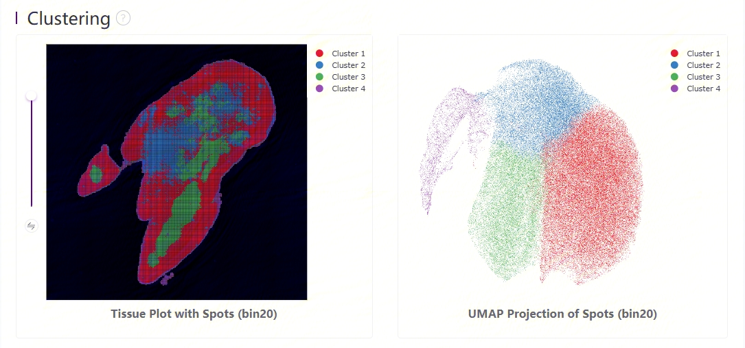
Clustering & UMAP
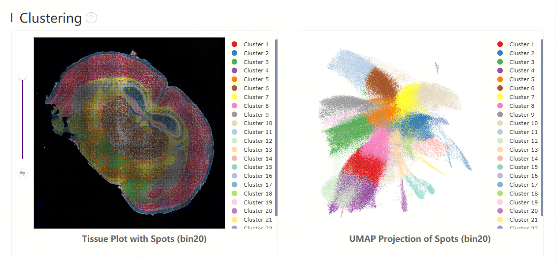
Leiden clustering and UMAP projection
Clustering is performed based on SN.tissue.gef using the Leiden algorithm. UMAP projections are performed based on SN.tissue.gef and colored by automated clustering. The same color is assigned to spots that are within a shorter distance and with similar gene expression profiles.
Differential expression analysis
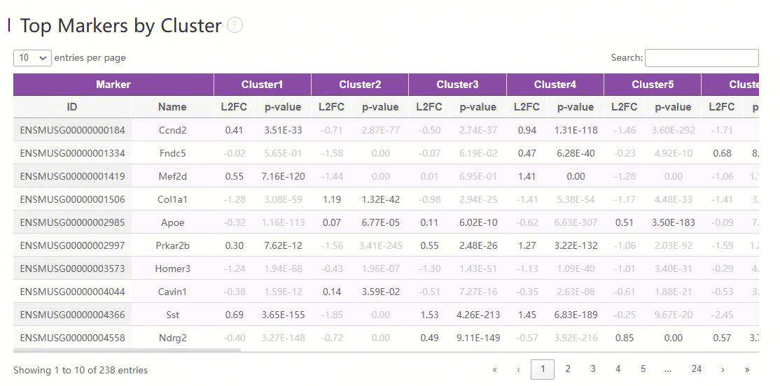
Marker feature table
The goal of the differential expression analysis is to identify markers that are more highly expressed in a cluster than the rest of the sample. For each marker, a differential expression test was run between each cluster and the remaining sample. An estimate of the log2 ratio of expression in a cluster to that in other coordinates is Log2 fold-change (L2FC). A value of 1.0 denotes a 2-fold increase in expression within the relevant cluster. Based on a negative binomial test, the p-value indicates the expression difference's statistical significance. The Benjamini-Hochberg method has been used to correct the p-value for multiple testing. Additionally, the top N features by L2FC for each cluster were kept after features in this table were filtered by (Mean UMI counts > 1.0). Grayed-out features have an adjusted p-value >= 0.10 or an L2FC < 0. N (ranges from 1 to 50) is the number of top features displayed per cluster, which is set to limit the amount of table entries displayed to 10,000. N=%10,000/K^2 where K is the number of clusters. Click on a column to sort by that value, or search a gene of interest.
When the values of L2FC in the marker feature table are blank, "infinity" and "-infinity", the analysis results are normal. These conditions are well explained below.
The calculation of L2FC is related to the expression number of cells of a certain gene in the case group and the control group. Since the calculation of L2FC uses the natural logarithm as the base, when the expression relationship has extremely high or low values, the three special values, none, "inf" and "-inf", will appear. The screenshot below uses inf and a constant to make a simple demonstration.
.png)
An example in Notebook using Python
The p-values should be increasing as the list descends (with a maximum of 1), infinitely close to 0.
If you find that the p-value is 0 in the result table, it may be because the calculated differential expression feature is extremely significant, leading to an extremely small p-value. This can exceed the limit of the data type (usually float64, depending on the basic computing package), resulting in a situation that cannot be expressed in scientific notation.
Cell Bin
This page contains results of statistics, plots, clustering, UMAP, and differential expression analysis, at cellbin dimension. Cell border expanding is automatically performed during SAW count and SAW realign, which means the contents of "Cell Bin" tab are based on SN.adjusted.cellbin.gef.
When it comes to --adjusted-distance=0 in SAW realign, all contents of this tab are based on SN.cellbin.gef.
Statistics
.PNG)
Detailed statistics of cellbin
The above table records the statistics of cellbin:
| Item | Description |
|---|---|
| Cell Count | Number of cells. |
| Mean Cell Area | Mean cell area, in pixes. |
| Median Cell Area | Median cell area, in pixes. |
| Mean Gene Type | Mean gene types per cell. |
| Median Gene Type | Median gene types per cell. |
| Mean MID | Mean MID count per cell. |
| Median MID | Median MID count per cell. |
Plots
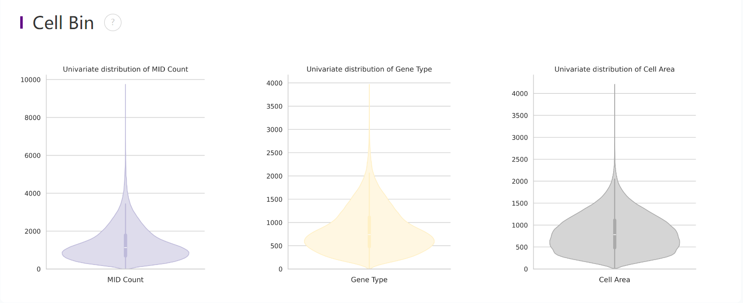
Distribution plots of MID and gene type
Violin plots show the distribution of deduplicated MID count, gene types and cell area in the cellbin.
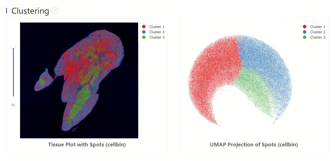
Clustering & UMAP
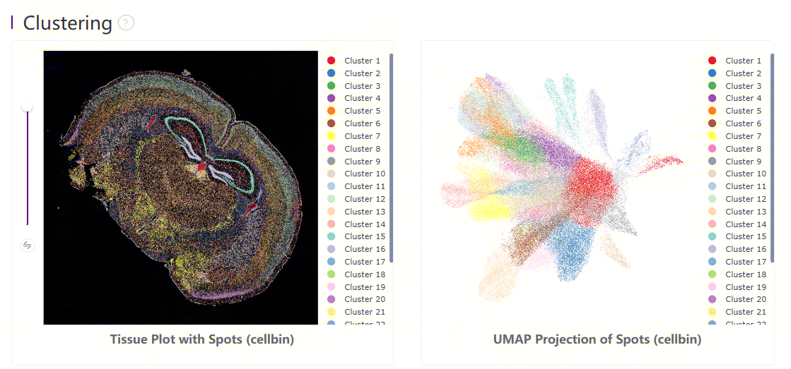
Leiden clustering and UMAP projection
Clustering is performed based on SN.adjusted.cellbin.gef or SN.cellbin.gef, using the Leiden algorithm. UMAP projections are performed based on SN.adjusted.cellbin.gef or SN.cellbin.gef, and colored by automated clustering. The same color is assigned to spots that are within a shorter distance and with similar gene expression profiles.
Differential expression analysis
.PNG)
Marker feature table
The goal of the differential expression analysis is to identify markers that are more highly expressed in a cluster than the rest of the sample. For each marker, a differential expression test was run between each cluster and the remaining sample. An estimate of the log2 ratio of expression in a cluster to that in other coordinates is Log2 fold-change (L2FC). A value of 1.0 denotes a 2-fold increase in expression within the relevant cluster. Based on a negative binomial test, the p-value indicates the expression difference's statistical significance. The Benjamini-Hochberg method has been used to correct the p-value for multiple testing. Additionally, the top N features by L2FC for each cluster were kept after features in this table were filtered by (Mean UMI counts > 1.0). Grayed-out features have an adjusted p-value >= 0.10 or an L2FC < 0. N (ranges from 1 to 50) is the number of top features displayed per cluster, which is set to limit the amount of table entries displayed to 10,000. N=%10,000/K^2 where K is the number of clusters. Click on a column to sort by that value, or search a gene of interest.
Interpretation for exceptional cases related to differential expression analysis can be found under Square Bin part.
Image information
Basic information about the microscopic staining image, usually involving microscope settings.
QC
| Metric | Description |
|---|---|
| Image QC version | The version of image QC module. |
| QC Pass | Whether the image(s) passed image QC quality check. |
| Trackline Score | Reference score for trackline detection. |
Stitching
| Metric | Description |
|---|---|
| Template Source Row No. | The row number of the template FOV used for predicting the entire template. |
| Template Source Column No. | The column number of the template FOV used for predicting the entire template. |
| Global Height | Height of the stitched image. |
| Global Width | Width of the stitched image. |
Registration
| Metric | Description |
|---|---|
| ScaleX | The lateral scaling between image and template. |
| ScaleY | The longitudinal scaling between image and template. |
| Rotation | The rotation angle of the image relative to the template. |
| Flip | Whether the image is flipped horizontally. |
| Image X Offset | Offset between image and matrix in x direction. |
| Image Y Offset | Offset between image and matrix in y direction |
| Counter Clockwise Rotation | Counter clockwise rotation angle. |
| Manual ScaleX | The lateral scaling based on image center (manual-registration). |
| Manual ScaleY | The longitudinal scaling based on image center (manual-registration). |
| Manual Rotation | The rotation angle based on image center (manual-registration). |
| Matrix X Start | Gene expression matrix offset in x direction by DNB numbers. |
| Matrix Y Start | Gene expression matrix offset in y direction by DNB numbers. |
| Matrix Height | Gene expression matrix height. |
| Matrix Width | Gene expression matrix width. |
Microorganism
Here is an another FFPE tissue sample of mouse lung which is especially for microorganism analysis.
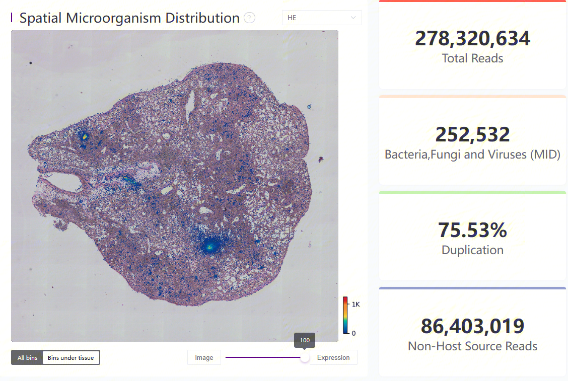
Microorganism heatmap under tissue region and four key metrics
The distribution plot of microorganism spatial expression, on the left, shows MID count at each bin20.
Denoising
| Metric | Description |
|---|---|
| Total Reads | Total number of input reads. (Ummapped Reads from transcriptome alignment) |
| Non-Host Source Reads | Number of reads that can not be aligned to the host genome. |
| Host Source Reads | Number of reads that can be aligned to the host genome during denoising. |
Taxonomic Classification
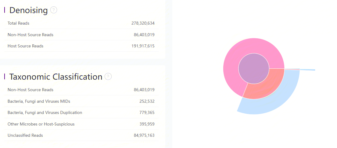
Mapping result of Bowtie2 and Kraken2
| Metric | Description |
|---|---|
| Non-Host Source Reads | Number of reads that can not be aligned to the host genome. |
| Bacteria, Fungi and Viruses MIDs | Number of unique mRNA molecular assigned to bacteria, fungi or viruses. |
| Bacteria, Fungi and Viruses Duplication | Number of assigned reads that have been corrected due to duplicated MID. |
| Other Microbes or Host-Suspicious | Number of reads assigned to other microbes (exclude bacteria, fungi and viruses) or host. |
| Unclassified Reads | Number of unclassified reads. |
Microbes Proportion (Phylum)
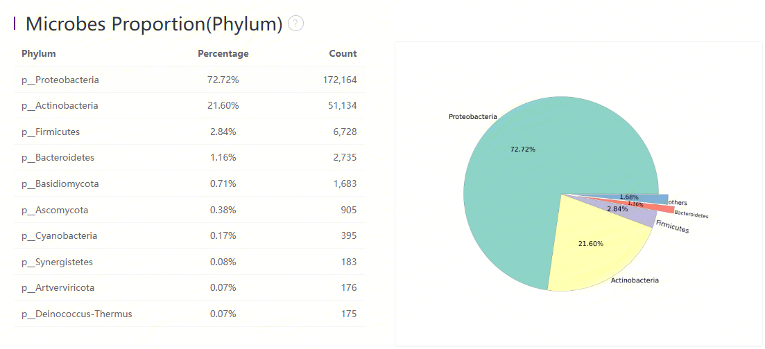
Microbes proportion at phylum level
The main proportion of microbes at the phylum level.
*the same for other classifications
Summary-Protein
.PNG)
.PNG)
The spatial protein expression distribution plot, containing all bins and bins under tissue, on the left, shows MID count at each bin20.
Total Reads is the total sequencing reads of input sequencing ADT FASTQs. Valid CID reads represents the number of reads with CIDs matching the mask file, with MIDs passing QC. Valid PID reads represents the number of reads that are mapped to the PID sequence in the protein panel. Unique PID reads represents the total number of unique protein reads (PID reads whose MIDs are different).
Key metrics
Key metrics of the data are listed:
| Metrics | Description |
|---|---|
| Total Reads | Total number of sequenced reads |
| Valid CID Reads | Number of reads with CIDs matching the mask file and with MIDs passing QC |
| Invalid CID Reads | Number of reads with CIDs that cannot be matched with the mask file |
| Valid PID Reads | Valid CID reads that mapped to the protein sequence in the protein sequence database (protein panel) |
| Invalid PID Reads | Valid CID reads that can not be mapped to the protein sequence in the protein sequence database (protein panel) |
| Unique PID Reads | Total number of unique protein reads (PID reads whose MIDs are different) |
| Sequencing Saturation | Number of PID reads with duplicated MID |
Sequencing saturation
.PNG)
The saturation analysis in the HTML report can assess the overall quality of the sequencing data. In order to improve calculation efficiency, small samples are randomly selected from successfully annotated reads in the bin20 or bin50 dimension. Therefore, the results of multiple runs of the same data may vary slightly. The formulas may not be identical, but the general shape of the curve is consistent.
- Figure 1: Curves fitted based on Unique Reads data from randomly sampled samples.
- Figure 2: Statistics of Unique Reads (reads with unique CID, PID and MID) in the sampled samples, saturation value = 1-(Unique Reads)/(Valid PID Reads), as the sampling volume increases, the fitting curve becomes near-flat, indicating that the data tends to be saturated. Whether to add additional tests depends on the overall project design and sample conditions. For example, it is recommended that additional tests be performed on precious samples. The threshold value of 0.8 in the report serves as a reminder for recommended guidance.
Protein correlations
Spearman correlation (in bin20 or bin50) between raw antibody counts under tissue, except isotype. Antibodies are clustered based on Spearman correlation coefficient.
.PNG)
Gene : protein correlations
Spearman correlation (in bin20 or bin50) between raw gene counts and raw antibody counts under tissue, where antibody has at least one marker gene in the protein panel.

Histogram of portein counts
Distribution of spot numbers vs log-scaled MID count (in bin20 or bin50).
.PNG)
Information
This item displays the basic information of the input FASTQs,
Species is from the --organism parameter used in SAW count, usually referring to the species.
Tissue is from the --tissue parameter used in SAW count.
Reference means the reference genome used in SAW count, as the same as Organism.
FASTQ records FASTQ files in SAW count, including file prefixes of all input sequencing ADT FASTQs.
Square Bin-Protein
This page contains results of statistics, plots, clustering, UMAP, and differential expression analysis, at bin dimension. Results come from the analysis based on <SN>.protein.tissue.gef file.
Statistics
| Item | Description |
|---|---|
| Bin Size | The size of Bin which is the unit of aggregated DNBs in a squared region. i.e. Bin 50 = 50 * 50 DNBs |
| Mean Reads (per bin) | Mean number of sequenced reads divided by the number of bins under tissue coverage. |
| Median Reads (per bin) | Median number of sequenced reads divided by the number of bins under tissue coverage (pick the middle value after sorting). |
| Mean MID (per bin) | Mean number of MIDs divided by the number of bins under tissue coverage. |
| Median MID (per bin) | Median number of MIDs divided by the number of bins under tissue coverage |
Plots
Violin plots show the distribution of deduplicated MID count in each bin.
Clustering & UMAP
Clustering is performed based on SN.protein.tissue.gef using the Leiden algorithm. UMAP projections are performed based on SN.protein.tissue.gef and colored by automated clustering. The same color is assigned to spots that are within a shorter distance and with similar gene expression profiles.
Cell Bin-Protein
This page contains results of statistics, plots, clustering, UMAP, and differential expression analysis, at cellbin dimension. Cell border expanding is automatically performed during SAW count and SAW realign, which means the contents of "Cell Bin" tab are based on SN.protein.adjusted.cellbin.gef.
When it comes to --adjusted-distance=0 in SAW realign, all contents of this tab are based on SN.protein.cellbin.gef.
Statistics
.PNG)
The above table records the statistics of cellbin:
| Item | Description |
|---|---|
| Cell Count | Number of cells. |
| Mean Cell Area | Mean cell area, in pixes. |
| Median Cell Area | Median cell area, in pixes. |
| Mean MID | Mean MID count per cell. |
| Median MID | Median MID count per cell. |
Plots
Violin plots show the distribution of deduplicated MID count and cell area in the cellbin.
Clustering & UMAP
Leiden clustering and UMAP projection
Clustering is performed based on SN.protein.adjusted.cellbin.gef or SN.protein.cellbin.gef, using the Leiden algorithm. UMAP projections are performed based on SN.protein.adjusted.cellbin.gef or SN.protein.cellbin.gef, and colored by automated clustering. The same color is assigned to spots that are within a shorter distance and with similar gene expression profiles.
Analysis (no longer available since 8.1.2)
This page contains results of clustering from gene-protein joint analysis, marker selection, and correlation between genes and proteins.
Multiomics clustering & UMAP
Clustering and UMAP projections are performed based on the latent space generated by totalVI.
Top markers by cluster
Heatmaps of top <=3 gene and protein markers per Leiden cluster from gene-protein jointly analysis. These features are filtered after one-vs-all differential expression analysis, following these rules:
- For gene, Bayes factor > 1 and expression proportion greater than 10% in the cluster;
- For protein, Bayes factor > 0.7.
Alerts
Thresholds are set for several important statistical indicators. If the analysis results are abnormal, an alert message will be displayed at the top of the HTML report.
Here is an abnormal exmple data just for display.
.png)
Alert information